Learn Data Frames in Pandas With Example

Learn Data Frames in Pandas With Example –

A DataFrame in Pandas is a two-dimensional labelled data structure with columns that can be of different data types. It is similar to a table in a relational database or a spreadsheet in which data is organized in rows and columns.

Learn Data Frames in Pandas With Example

Advantages of Using Data Frames

Data frames are a tabular data structure used in various programming languages for handling and analyzing structured data. Here are some advantages of using data frames:

Structured Representation: Data frames provide a structured way to represent and organize data in a tabular format. This makes it easy to understand and work with data, especially when dealing with multiple variables or attributes.
Columnar Operations: Data frames allow for efficient column-wise operations, making it easy to perform computations or manipulations on specific variables without having to iterate through each element individually. This can significantly improve performance and readability of code.
Integration with Statistical Packages: Data frames are commonly used in statistical programming languages like R and Python (with libraries like Pandas). They seamlessly integrate with statistical packages and libraries, making it easy to perform data analysis, visualization, and modeling.
Data Cleaning and Transformation: Data frames provide built-in functions and methods for cleaning and transforming data. This includes handling missing values, filtering rows based on conditions, and transforming data types, making the data preparation process more straightforward.
Indexing and Subsetting: Data frames support indexing and subsetting operations, allowing users to access and manipulate specific portions of the data easily. This is crucial for selecting relevant subsets for analysis or visualization.
Data Alignment: In data frames, columns are aligned based on their index, which ensures that operations are performed on corresponding elements. This alignment simplifies code and prevents common errors that might arise when working with mismatched data.
Ease of Import and Export: Data frames facilitate the import and export of data from various file formats, including CSV, Excel, SQL databases, and more. This makes it easy to work with data from different sources and systems.
Support for Time Series Data: Data frames often include features for handling time series data, such as date-time indexing and functions for time-based operations. This is crucial for analyzing data with temporal components.
Wide Range of Functions: Data frames come with a rich set of functions for data manipulation, exploration, and analysis. This includes aggregation functions, statistical summaries, and descriptive statistics, which are essential for understanding the characteristics of the data.
Interoperability: Data frames provide a common data structure that is widely supported across various libraries and tools in the data science ecosystem. This interoperability makes it easy to transition between different stages of the data analysis pipeline and collaborate with others.

In summary, data frames offer a versatile and efficient way to handle and analyze structured data, providing numerous advantages for data scientists, analysts, and programmers working on data-related tasks.

Different Methods To Create Data Frame in Python Pandas

Creating a DataFrame in pandas can be done in various ways, but one of the most common methods is using the pd.DataFrame() constructor. Here are a few examples:

Example 1: Creating a DataFrame from a Dictionary

Here’s an example of creating and working with a DataFrame in Pandas:

import pandas as pd
# Creating a DataFrame from a dictionary
data = {
    'Name': ['Alice', 'Bob', 'Charlie'],
    'Age': [25, 30, 35],
    'City': ['New York', 'San Francisco', 'Los Angeles']
}
df = pd.DataFrame(data)
# Displaying the DataFrame
print("Original DataFrame:")
print(df)

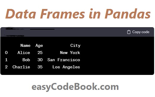
Output:

      Name  Age           City
0    Alice   25       New York
1      Bob   30  San Francisco
2  Charlie   35    Los Angeles

This will create a DataFrame with three columns: ‘Name’, ‘Age’, and ‘City’.

In this example:

Creating and Displaying a Data Frame in Pandas

Importing Pandas: The import pandas as pd statement imports the Pandas library and aliases it as pd for convenience.
Creating a DataFrame: The pd.DataFrame() constructor is used to create a DataFrame from a dictionary (data). Keys of the dictionary become column names, and values become the data in each column.
Displaying the DataFrame: The print(df) statement prints the DataFrame to the console.

Example 2: Creating a DataFrame from a List of Lists

import pandas as pd

# Creating a DataFrame from a list of lists
data_list = [
    ['Alice', 25, 'New York'],
    ['Bob', 30, 'San Francisco'],
    ['Charlie', 35, 'Los Angeles']
]

df = pd.DataFrame(data_list, columns=['Name', 'Age', 'City'])
print(df)

Here, we explicitly specify the column names using the columns parameter.

Example 3: Creating an Empty DataFrame and Adding Rows

import pandas as pd

# Creating an empty DataFrame
df = pd.DataFrame(columns=['Name', 'Age', 'City'])

# Adding rows to the DataFrame
df = df.append({'Name': 'Alice', 'Age': 25, 'City': 'New York'}, ignore_index=True)
df = df.append({'Name': 'Bob', 'Age': 30, 'City': 'San Francisco'}, ignore_index=True)
df = df.append({'Name': 'Charlie', 'Age': 35, 'City': 'Los Angeles'}, ignore_index=True)

print(df)

Here, we create an empty DataFrame and use the append method to add rows to it.

Example Python Code for Common Operations on Data Frame

# Accessing columns
print("\nAccessing 'Name' column:")
print(df['Name'])

# Accessing rows
print(“\nAccessing the second row:”)
print(df.iloc[1])

# Descriptive statistics
print(“\nDescriptive statistics:”)
print(df.describe())

# Adding a new column
df[‘Salary’] = [50000, 60000, 75000]
print(“\nDataFrame with ‘Salary’ column added:”)
print(df)

# Filtering data
print(“\nFiltering based on age:”)
print(df[df[‘Age’] > 30])

Output:

Accessing 'Name' column:
0      Alice
1        Bob
2    Charlie
Name: Name, dtype: object

Accessing the second row:
Name                Bob
Age                  30
City    San Francisco
Name: 1, dtype: object

Descriptive statistics:
        Age        Salary
count   3.0      3.000000
mean   30.0  61666.666667
std     5.0  12291.864875
min    25.0  50000.000000
25%    27.5  55000.000000
50%    30.0  60000.000000
75%    32.5  67500.000000
max    35.0  75000.000000

DataFrame with 'Salary' column added:
      Name  Age           City  Salary
0    Alice   25       New York   50000
1      Bob   30  San Francisco   60000
2  Charlie   35    Los Angeles   75000

Filtering based on age:
      Name  Age         City  Salary
2  Charlie   35  Los Angeles   75000

These examples demonstrate basic DataFrame operations, including accessing columns and rows, descriptive statistics, adding a new column, and filtering data. Pandas provides a rich set of functionality for data manipulation, analysis, and visualization, making it a powerful tool for working with structured data.

Example 2 for Using Data Frames in Pandas

Let’s create another example with a different DataFrame. In this example, I’ll use data related to employee information:

import pandas as pd

# Creating a DataFrame from a list of dictionaries
employee_data = [
    {'Name': 'Alice', 'Age': 28, 'Department': 'HR', 'Salary': 60000},
    {'Name': 'Bob', 'Age': 35, 'Department': 'Engineering', 'Salary': 75000},
    {'Name': 'Charlie', 'Age': 30, 'Department': 'Marketing', 'Salary': 70000},
    {'Name': 'David', 'Age': 25, 'Department': 'HR', 'Salary': 55000},
]

employee_df = pd.DataFrame(employee_data)

# Displaying the DataFrame
print("Employee DataFrame:")
print(employee_df)

Output:

Employee DataFrame:
      Name  Age   Department  Salary
0    Alice   28           HR   60000
1      Bob   35  Engineering   75000
2  Charlie   30    Marketing   70000
3    David   25           HR   55000

Now, let’s perform some operations on this employee DataFrame:

# Accessing columns
print("\nAccessing 'Name' and 'Department' columns:")
print(employee_df[['Name', 'Department']])

# Descriptive statistics
print("\nDescriptive statistics:")
print(employee_df.describe())

# Adding a new column
employee_df['Bonus'] = [5000, 7500, 7000, 4500]
print("\nEmployee DataFrame with 'Bonus' column added:")
print(employee_df)

# Filtering data
print("\nFiltering based on department (HR):")
print(employee_df[employee_df['Department'] == 'HR'])